PhINs Tutorial Tests Recovery of Hidden Pharmacological Dynamics

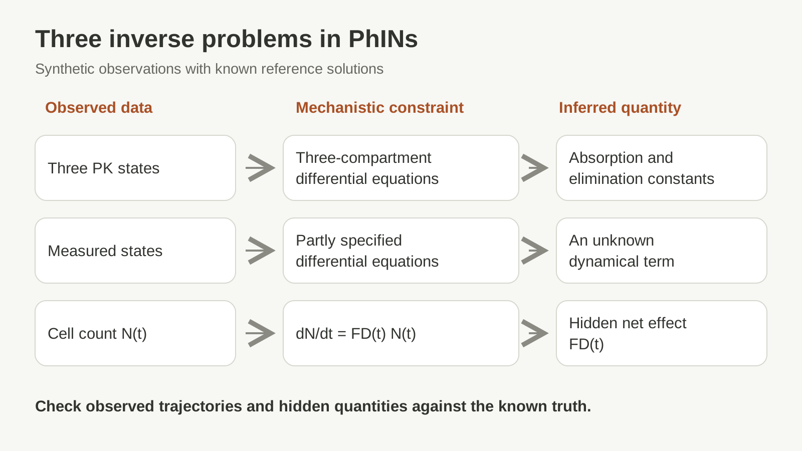
Equations constrain the learning problem

PhINs, short for Pharmacometrics-Informed Networks, is a software library presented in a tutorial by researchers at Brown University and the University of Waterloo. It combines observed trajectories with known differential equations to estimate parameters or dynamics that cannot be measured directly. The examples address pharmacokinetics, pharmacodynamics and quantitative systems pharmacology, using synthetic data whose true generating mechanisms are available for checking the inference.

A physics-informed neural network learns trajectories while penalizing violations of the governing equations and initial conditions. The tutorial compares conventional multilayer perceptrons with Kolmogorov–Arnold networks, an alternative representation that learns functions along network connections. Their physics-informed implementations are called PINNs and PIKANs, respectively. The shared interface reuses the mechanistic residual, data bundle and constraints across these representations.

Three increasingly hidden quantities

The first worked example uses three compartments for gastrointestinal drug amount, central drug amount and eliminated drug. Observations of all three states constrain two unknown transfer-rate constants. The synthetic reference values are 0.72 h−1 for absorption and 0.15 h−1 for elimination. The baseline setting samples 50 times over 50 hours, with controlled measurement noise. Both architectures recover the compartmental trajectories and rate constants, while reducing the observation count makes recovery more sensitive, particularly for the absorption constant.

The second example changes the question from estimating fixed constants to learning an unknown term in an otherwise specified equation system. This is a gray-box problem: part of the dynamics is supplied by mechanistic knowledge and part must be inferred. Its known synthetic function provides an independent target for evaluating whether the network has recovered the missing term, in addition to reproducing the measured states.

The third example provides only a synthetic cancer-cell-count trajectory. A hidden time-varying function describes the net change in cell number, incorporating proliferation, drug-induced death and the cell-number constraint of the generating model. The network reconstructs the observed count and this hidden function over a 600-hour interval. The study compares different observation densities, residual-sampling strategies and loss-weighting schemes.

The hidden function is small in magnitude, so its learned output is scaled by 0.03 when used in the differential equation. An additional initial-value constraint helps anchor the otherwise indirect inference. These details matter because a smooth, accurate fit to cell number alone could coexist with an inaccurate or weakly identified hidden function.

Recovery depends on sampling and training

Table 3 reports errors separately for observed cell count and hidden net effect. With 120 observations and 5% noise, the PINN configuration had root-mean-square errors of 7.78 × 10−3 for cell count and 8.12 × 10−4 for the hidden function. The corresponding PIKAN configuration had errors of 3.89 × 10−3 and 4.70 × 10−4. Other rows show that performance changes with observation density, architecture and training strategy; the table does not establish one architecture as uniformly superior.

The tutorial also distinguishes numerical verification from biological validation. Residual diagnostics and forward simulation with an ordinary differential equation solver can test consistency of the inferred quantities. Comparison with synthetic ground truth tests recovery in the controlled example. A pharmacological application would additionally need to establish that the chosen equations and observation model describe the relevant biological system.

Identifiability remains a separate requirement

Mechanistic constraints can regularize learning, but they cannot create information missing from the observations. Several parameter combinations or hidden functions may explain the same trajectory. The authors therefore place identifiability analysis, uncertainty, biological plausibility and held-out-condition checks alongside the training loss.

The supplied code and notebooks make the three examples reproducible as tutorial problems. Their controlled noise, regular sampling and known generating equations leave severe sparsity, irregular clinical measurements, repeated-dose discontinuities and model misspecification as further challenges. The authors position these networks alongside established estimation methods, with uncertainty quantification and population-level variability among the development areas for pharmacometric applications.